Examples

%matplotlib inline

import numpy as np
import scipy as sp
import scipy.cluster.hierarchy
from scipy.spatial.distance import pdist, squareform

from sklearn import datasets

import matplotlib as mpl
import matplotlib.pyplot as plt
from mpl_toolkits.mplot3d import Axes3D
mpl.rcParams.update({'font.size': 16})

import sys
sys.path.append('../../')
from pyprotoclust import protoclust

def axlabel(ax, xlabel, ylabel, zlabel=None, params={}):
    ''' Shorthand for axis labelling '''
    ax.set_xlabel(xlabel, **params)
    ax.set_ylabel(ylabel, **params)
    if zlabel:
        ax.set_zlabel(zlabel, **params)
    return ax

def fancy_dendrogram(ax, *args, **kwargs):
    ''' Nicer plotting of dendrograms courtesy of https://joernhees.de/blog/ '''
    title = ''
    max_d = kwargs.pop('max_d', None)
    if max_d and 'color_threshold' not in kwargs:
        kwargs['color_threshold'] = max_d
    annotate_above = kwargs.pop('annotate_above', 0)

    ddata = sp.cluster.hierarchy.dendrogram(*args, **kwargs)

    if kwargs.get('truncate_mode', False):
        title = title + ', p={}'.format(kwargs.get('p', None))

    if not kwargs.get('no_plot', False):
        ax.set_title(title)
        ax.set_ylabel('distance')
        for i, d, c in zip(ddata['icoord'], ddata['dcoord'], ddata['color_list']):
            x = 0.5 * sum(i[1:3])
            y = d[1]
            if y > annotate_above:
                ax.plot(x, y, 'o', c=c)
        if max_d:
            ax.axhline(y=max_d, c='k', ls='--')
    return ddata

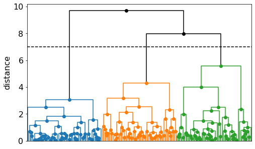
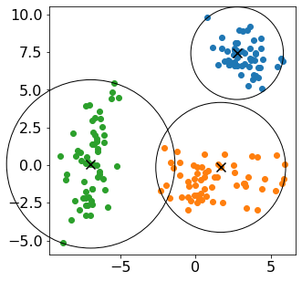
Gaussians in 2D

This example shows how the cut height is related to the within-cluster variance.

n = 60
np.random.seed(4)

examples = [{'mean': [-7, 0], 'cov': [[1, 1], [1, 5]]},
            {'mean': [1, -1], 'cov': [[5, 0], [0, 1]]},
            {'mean': [3, 7], 'cov': [[1, 0], [0, 1]]}]
data = np.vstack([np.random.multivariate_normal(i['mean'], i['cov'], n) for i in examples])

# Produce clustering
Z, prototypes = protoclust(squareform(pdist(data)), verbose=True, notebook=True)
Z = np.array(Z)
prototypes = np.array(prototypes)

cut_height = 7

# Get clusters associated with the cut height
T = sp.cluster.hierarchy.fcluster(Z, cut_height, criterion='distance')
L,M = sp.cluster.hierarchy.leaders(Z, T)

# Set the default color map
cmap = plt.cm.get_cmap('tab10', 10)
sp.cluster.hierarchy.set_link_color_palette([mpl.colors.to_hex(cmap(k-1)) for k in np.unique(T)])

# Plot dendrogram with a specific cut height
fig,ax = plt.subplots(1, figsize=[8,5])
fancy_dendrogram(ax, Z, max_d=cut_height, above_threshold_color='k')
ax.set_xticks([])

# Plot data
fig,ax = plt.subplots(1, figsize=[5,5])
ax.set_aspect('equal')
for i in range(3):
    ax.scatter(data[i*n:(i+1)*n,0], data[i*n:(i+1)*n,1], color=cmap(T[i*n]-1))

# Plot prototypes with cut heights as circles
centers = data[prototypes[L]]
ax.scatter(*centers.T, c='k', marker='x', s=100)
for xy, r in zip(centers, Z[L-len(data), 2]):
    ax.add_artist(mpl.patches.Circle(xy, radius=r, fill=False, clip_on=False))

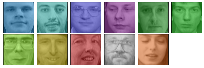
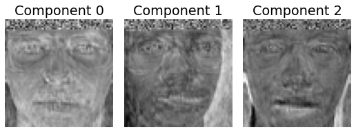
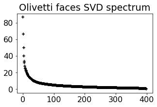
Olivetti Faces

This example shows how the method naturally lends itself to datasets where image representatives of clusters are desirable.

# Load faces
faces = datasets.fetch_olivetti_faces()
X = faces.data
n,d = X.shape # d = 64x64 = 4096
Y = faces.target

# Compute SVD
U,S,Vt = np.linalg.svd(X - np.mean(X, axis=0))

# Plot SVD basis
fig, ax = plt.subplots(1, 3, figsize=[9,3])
fig.subplots_adjust(wspace=0.1)

for i in range(3):
    ax[i].imshow(Vt[:,i].reshape(64,64), cmap='gray')
    ax[i].axis("off")
    ax[i].set_title('Component {}'.format(i))

# Plot SVD spectrum
fig, ax = plt.subplots(1, figsize=[5,3])
ax.set_title('Olivetti faces SVD spectrum')
ax.scatter(list(range(len(S))), S, marker='+', c='k')

downloading Olivetti faces from https://ndownloader.figshare.com/files/5976027 to /home/docs/scikit_learn_data

<matplotlib.collections.PathCollection at 0x7f7200f98f10>

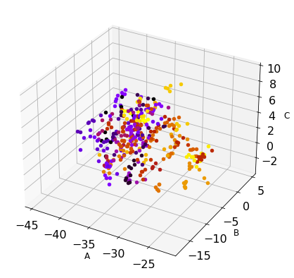
# Plot projected coordinates and color by label
fig= plt.figure(figsize=[9,7])
ax = fig.add_subplot(111, projection='3d')
pcX = X@Vt.T[:,:3]
cmap = plt.cm.get_cmap('gnuplot', len(np.unique(Y)))
for i,j,k,c in zip(pcX[:,0], pcX[:,1], pcX[:,2], Y):
    ax.scatter(i,j,k,color=cmap(c))
axlabel(ax, 'A','B','C', {'fontsize': 12});

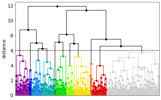
# Cluster
Z, prototypes = protoclust(squareform(pdist(pcX)), verbose=True, notebook=True)
prototypes = np.array(prototypes)

cut_height = 6

T = sp.cluster.hierarchy.fcluster(Z, cut_height, criterion='distance')
indices,_ = sp.cluster.hierarchy.leaders(Z,T)

# Discretize color map based on cluster number
cmap = plt.cm.get_cmap('nipy_spectral', len(np.unique(T))+1)
sp.cluster.hierarchy.set_link_color_palette([mpl.colors.to_hex(cmap(k)) for k in np.unique(T)])

# Plot 1: dendrogram
fig,ax  = plt.subplots(1, figsize=[9,6])
fancy_dendrogram(ax, Z, max_d=cut_height, above_threshold_color='k')
ax.set_xticks([]);

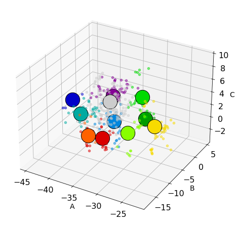
# Plot 2: Projected clusters
fig= plt.figure(figsize=[10,8])
ax = fig.add_subplot(111, projection='3d')

# Project onto the principle components from the SVD
pcX = X@Vt.T[:,:3]

# Plot faces in this reduced space
for index, row in enumerate(pcX):
    ax.scatter(*row, color=cmap(T[index]), alpha=0.5)

for p in prototypes[indices]:
    ax.scatter(*pcX[p, :], edgecolor='k', facecolor=cmap(T[p]), s=800, marker='o')

axlabel(ax, 'A','B','C', {'fontsize': 14});

# Plot 3: Prototypes
fig, axes = plt.subplots(2,len(indices)//2+1, figsize=[12,4])
fig.subplots_adjust(wspace=.1, hspace=0)
for i,iax in enumerate(axes.flatten()):
    if i < len(indices):
        p = prototypes[indices[i]]
        c = cmap(T[p])
        iax.set_xticks([])
        iax.set_yticks([])
        iax.set_facecolor(c)
        im = X[p].reshape(64,64)
    else:
        im = np.ones([64,64])
        iax.axis('off')
    iax.imshow(im, alpha=0.6, cmap='gray', vmin=0, vmax=1)